Approach and model formulation
A population-based deterministic approach was used to model the transmission of malaria. The mathematical model consisted of variable human and mosquito populations. The human and mosquito populations were divided into compartments. Infection dynamics in humans were described by ordinary differential equations and used the epidemiological compartment modelling approach as follows: individuals start life being susceptible to falciparum malaria infection (Sh); and these are then exposed at a certain probability to infectious mosquito bites. The exposed (Eh) compartment consists of individuals who are infected but are not capable of infecting others during a latent period. The infectious humans (Ih) give rise to more infected mosquitoes through their interaction with the susceptible mosquitoes. Once treated, individuals recover (Rh) from the disease with partial immunity and after some time they become susceptible again (SEIR). Although the recovered are not at an immediate risk of developing clinical disease, however, they can still infect susceptible mosquitoes but at a lower rate than that of infectious individuals [19].
Infection dynamics in mosquito vectors followed the SEI pattern of compartimentalisation: susceptible mosquitoes (Sv) get infected at a certain probability when they get a blood meal either from infectious humans or recovered humans; then move to exposed compartment (Ev) and finally the infectious compartment (Iv). The recovered class is here omitted for the mosquito population because once infected the mosquito remains so until death.
The adapted SEIR model was based on Ngwa and Shu [9]. The SEIR model of compartmentalization (Figure 1 was chosen because it is more realistic as it includes the latent phase (exposed class) which is not found in SIR or SIS models.
In the Ngwa and Shu model [9], humans follow an SEIR pattern while mosquitoes follow the SEI pattern of compartmentalization. Infectious humans either recover with or without immunity; and those who recover with partial immunity remain infectious while those who recover without immunity return directly to the susceptible compartment. The modeling approach adopted in this research is a modification of the Ngwa and Shu model capturing variable human and mosquito populations, preventive intervention measures such as Long-Lasting Insecticidal Nets (LLINS), immigration, recovery with temporary immunity and disease-induced death in humans. The direct infectious-to-susceptible transfer that the Ngwa and Shu model contains is excluded from the model, because most people show some varying periods of immunity before becoming susceptible again [19]. Interaction between the two populations is as shown in Figure 1.
Description of model parameters
With reference to Figure 1, Table 1 provides descriptions of the parameters used in the malaria model.
Model assumptions
Model equations
In view of the model assumptions above and the schematic diagram in Figure 1, the dynamics of malaria transmission was described by the following model equations: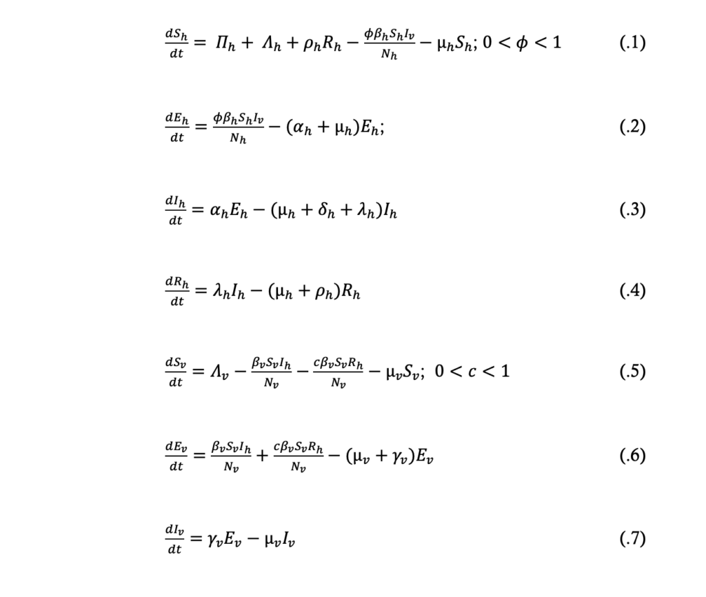
From the model equations (.1) to (.4) the total population size, Nh, at time t is given by:

From the model equations (.5) to (.7) the total population size, Nv, at time t is given by:

Model fitting, validation and parameter estimation
A least-squares estimation method in Microsoft excel 2019 was used to fit the model system (.1) to (.7). Model calibration was done using the full dataset from 2015 – 2020. The dataset for December 2020 – February 2021 was used to assess and strengthen the model’s predictive abilities. Parameter estimation and model simulation were carried out in Microsoft excel 2019.
The disease-free equilibrium point was determined and the local stability of the system was described in terms of the threshold parameter, the basic reproduction number (R0), which was obtained using the next generation matrix method.
Existence of the disease-free equilibrium (DFE) point
The DFE point are steady state solutions where there is no malaria in the human population, and no plasmodium parasites in mosquitoes. Thus the DFE point, given by E0hv (Sh,Eh,Ih,Rh;Sv,Ev,Iv) of the system of differential equations .1 to .7, is obtained by solving the equation

The “infected” classes in the human or mosquito populations are either the exposed or infectious, that is \( E_h, I_h, R_h, E_v, I_v \). So in the absence of disease, at the DFE point of the system (.1) to (.7), it implies \( E_h = I_h = R_h = E_v = I_v = 0 \); \( S_h = \frac{\Pi_h + \Delta_h}{\mu_h} \), and \( S_v = \frac{\Delta_v}{\mu_v} \)
Thus the DFE point \( E_{0hv}(S_h, E_h, I_h, R_h, S_v, E_v, I_v) \) is given by
\( E_{0hv} \left( \frac{\Pi_h + \Delta_h}{\mu_h}, 0, 0, 0; \frac{\Delta_v}{\mu_v}, 0, 0 \right) \).
As such, the positive feasible region of the system for the human population, equations (.1) to (.4) is given by
$$ \{(S_h,E_h,I_h,R_h ): S_h+E_h+I_h+R_h\leq \frac{\Pi_h+\Lambda_h}{\mu_h}, S_h>0,E_h\geq0,I_h\geq0,R_h\geq0\}. $$
The positive feasible region of the model equations (.5) to (.7) for the mosquito population is given by
$$ \{(S_v,E_v,I_v ): S_v+E_v+I_v\leq \frac{\Lambda_v}{\mu_v}, S_v>0,E_v\geq0,I_v\geq0\}. $$
It follows therefore that the DFE point, \( E_{0hv} \left( \frac{\Pi_h+\Lambda_h}{\mu_h} ,0,0,0; \frac{\Lambda_v}{\mu_v} ,0,0 \right) \), of the system of equations (.1) to (.7) is locally asymptotically stable if \( R_{0hv}<1 \) and unstable if \( R_{0hv}>1 \), where
$$ R_{0hv}=\sqrt{R_{0h} R_{0v}}. $$
The square root is as a result of the needed two generations for an infected vector or host to reproduce itself. \( R_{0hv} \) is the basic reproduction number of the system, while \( R_{0h} \) and \( R_{0v} \) are the basic reproduction numbers for human and mosquito populations, respectively.
The basic reproduction number, R0
The basic reproduction number, R0, is defined as the number of secondary infections that one infectious individual generates over the duration of his/ her entire infectious period, assuming that all the individuals in the population are susceptible.
When R0 < 1, each infected individual produces, on average, less than one new infected individual and hence it is expected that the disease will die out. On the other hand, if , each individual produces more than one new infected individual, so it would be expected that the disease will spread through the population. Therefore, the threshold condition for eliminating or eradicating the disease is to reduce the value of to less than one.
We introduce new variables in terms of proportion as follows:

Where
$$ s+e+i+r=1; \quad x+y+z=1; \quad (1.2b) $$
$$ s=(1-e-i-r), \quad \text{and} \quad x=(1-y-z); $$
$$ S_h=sN_h \quad \text{and} \quad S_v=xN_v. $$
Hence
$$ S_h=(1-e-i-r) N_h, \quad \text{and} \quad S_v=(1-y-z) N_v. \quad (1.2c) $$
Now from equations (1.2a), it can be seen that:
$$ N_h \frac{ds}{dt} = \frac{dS_h}{dt} – s \frac{dN_h}{dt} \quad (1.3a) $$
$$ N_h \frac{de}{dt} = \frac{dE_h}{dt} – e \frac{dN_h}{dt} \quad (1.3b) $$
$$ N_h \frac{di}{dt} = \frac{dI_h}{dt} – i \frac{dN_h}{dt} \quad (1.3c) $$
$$ N_h \frac{dr}{dt} = \frac{dR_h}{dt} – r \frac{dN_h}{dt} \quad (1.3d) $$
$$ N_v \frac{dx}{dt} = \frac{dS_v}{dt} – x \frac{dN_v}{dt} \quad (1.3e) $$
$$ N_v \frac{dy}{dt} = \frac{dE_v}{dt} – y \frac{dN_v}{dt} \quad (1.3f) $$
$$ N_v \frac{dz}{dt} = \frac{dI_v}{dt} – z \frac{dN_v}{dt} \quad (1.3g) $$
Using the relationships of equations (1.2) and (1.3), and re-writing the system equations (.1) to (.7) gives the following equations:
$$ \frac{ds}{dt} = a + b + \rho_h r – \phi \beta_h sz – (a + b – \delta_h i)s \quad (1.4) $$
$$ \frac{de}{dt} = \phi \beta_h sz – (a + b + \alpha_h – \delta_h i)e \quad (1.5) $$
$$ \frac{di}{dt} = \alpha_h e – (a + b + \delta_h + \lambda_h – \delta_h i)i \quad (1.6) $$
$$ \frac{dr}{dt} = \lambda_h i – (a + b + \rho_h – \delta_h i)r \quad (1.7) $$
$$ \frac{dx}{dt} = d – \beta_v xi – c\beta_v xr – dx \quad (1.8) $$
$$ \frac{dy}{dt} = \beta_v xi + c\beta_v xr – (\gamma_v + d)y \quad (1.9) $$
$$ \frac{dz}{dt} = \gamma_v y – dz \quad (1.10) $$
The infected classes of the system (.1) to (.7), and hence system (1.4) to (1.10), are now \( e, i, r, y, \) and \( z \). The next generation matrix method was used to determine the \( R_0 \) of the present model. The \( R_0 \) is taken to be the dominant eigenvalue of the next generation matrix. This is given by the matrix \( FV^{-1} \), where \( F \) represents the rate of appearance of new infections in the compartments and \( V \) represents the transfer of individuals in and out of compartments, and \( E_0 \) is the disease-free equilibrium point. Thus:
$$ F \begin{bmatrix} e \\ i \\ r \\ y \\ z \end{bmatrix} =
\begin{bmatrix} \phi \beta_h sz \\ 0 \\ 0 \\ \beta_v xi + c\beta_v xr \\ 0 \end{bmatrix} $$
$$ F(E_0) = \begin{bmatrix} 0 & 0 & 0 & 0 & \phi\beta_h \\ 0 & 0 & 0 & 0 & 0 \\ 0 & 0 & 0 & 0 & 0 \\ 0 & \beta_v & c\beta_v & 0 & 0 \\ 0 & 0 & 0 & 0 & 0 \end{bmatrix} $$
And
$$ V \begin{bmatrix} e \\ i \\ r \\ y \\ z \end{bmatrix} =
\begin{bmatrix} (a+b+\alpha_h – \delta_h i)e \\ -\alpha_h e + (a+b+\delta_h+\lambda_h – \delta_h i)i \\ -\lambda_h i + (a+b+\rho_h – \delta_h i)r \\ (d+\gamma_v )y \\ -\gamma_v y + dz \end{bmatrix} $$
$$ V(E_0) = \begin{bmatrix} (a+b+\alpha_h) & 0 & 0 & 0 & 0 \\ -\alpha_h & (a+b+\delta_h+\lambda_h) & 0 & 0 & 0 \\ 0 & -\lambda_h & (a+b+\rho_h) & 0 & 0 \\ 0 & 0 & 0 & (d+\gamma_v) & 0 \\ 0 & 0 & 0 & -\gamma_v & d \end{bmatrix} $$
Let
$$ a_{11} = (a+b+\alpha_h), \quad a_{21} = -\alpha_h, \quad a_{22} = (a+b+\delta_h+\lambda_h), \quad a_{32} = -\lambda_h, \quad a_{33} = (a+b+\rho_h), \quad a_{44} = (d+\gamma_v), \quad a_{54} = -\gamma_v, \quad a_{55} = d. $$
Then it implies:
$$ |V| = a_{11} a_{22} a_{33} a_{44} a_{55}. $$
Let \( V \) be a vector \( V \) as a matrix of its cofactors, it then implies:
$$ V = \begin{bmatrix} a_{22} a_{33} a_{44} a_{55} & -a_{21} a_{33} a_{44} a_{55} & a_{21} a_{32} a_{44} a_{55} & 0 & 0 \\ 0 & a_{11} a_{33} a_{44} a_{55} & -a_{11} a_{32} a_{44} a_{55} & 0 & 0 \\ 0 & 0 & a_{11} a_{22} a_{44} a_{55} & 0 & 0 \\ 0 & 0 & 0 & -a_{11} a_{22} a_{33} a_{54} & 0 \\ 0 & 0 & 0 & 0 & 0 \end{bmatrix} $$
Then
$$ V^T = \begin{bmatrix} a_{22} a_{33} a_{44} a_{55} & 0 & 0 & 0 & 0 \\ -a_{21} a_{33} a_{44} a_{55} & a_{11} a_{33} a_{44} a_{55} & 0 & 0 & 0 \\ a_{21} a_{32} a_{44} a_{55} & -a_{11} a_{32} a_{44} a_{55} & a_{11} a_{22} a_{44} a_{55} & 0 & 0 \\ 0 & 0 & 0 & 0 & 0 \\ 0 & 0 & 0 & -a_{11} a_{22} a_{33} a_{54} & 0 \end{bmatrix} $$
$$ V^{-1} = \frac{1}{|V|} V^T \quad (1.11) $$
$$ = \begin{bmatrix} \frac{1}{a_{11}} & 0 & 0 & 0 & 0 \\ \frac{-a_{21}}{a_{11} a_{22}} & \frac{1}{a_{22}} & 0 & 0 & 0 \\ \frac{a_{21} a_{32}}{a_{11} a_{22} a_{33}} & \frac{-a_{32}}{a_{22} a_{33}} & \frac{1}{a_{33}} & 0 & 0 \\ 0 & 0 & 0 & 0 & 0 \\ 0 & 0 & 0 & \frac{-a_{54}}{a_{44} a_{55}} & 0 \end{bmatrix} $$
Therefore, the basic reproduction number \( R_{0hv} \) is thus given by:
$$ R_{0hv} = \sqrt{R_{0h} R_{0v}} $$
Therefore:
$$
R_{0hv} = \sqrt{ \left( \left[ \frac{\alpha_h \beta_v}{(a+b+\alpha_h)(a+b+\delta_h+\lambda_h)} + \frac{c\beta_h \alpha_h \lambda_h}{(a+b+\alpha_h)(a+b+\delta_h+\lambda_h)(a+b+\rho_h)} \right] \cdot \left( \frac{\varphi \beta_h \gamma_v}{d(d+\gamma_v)} \right) \right) }
$$
$$
R_{0hv} = \sqrt{ \frac{\varphi \beta_h \gamma_v \left[ \alpha_h \beta_v (a+b+\rho_h) + c\beta_v \alpha_h \lambda_h \right]}{d(d+\gamma_v)(a+b+\alpha_h)(a+b+\delta_h+\lambda_h)(a+b+\rho_h)} }
$$
$$ R_{0hv} = \sqrt{\frac{\phi \beta_h \gamma_v [\alpha_h \beta_v (a+b+\rho_h) + c\beta_v \alpha_h \lambda_h]}{d(d+\gamma_v)(a+b+\alpha_h)(a+b+\delta_h+\lambda_h)(a+b+\rho_h)}} $$
$$ = 0.096906348 \quad \text{(from Table 4); } R_{0hv} < 1. $$
Malaria transmission is here depicted as resulting from transmission of the plasmodia parasites from infected humans to susceptible mosquitoes and from infected mosquitoes to susceptible humans. The \( R_{0hv} \) here is related to the transmission of disease by infectious humans in the \( I \) compartment, and/or partially immune recovered in the \( R \) compartment to susceptible mosquitoes. Susceptible humans are infected following infectious bites by infected mosquitoes.
Thus, near the DFE (\( E_{0hv} \)) point, each infected human is likely to produce:
$$
\frac{\beta_v \gamma_v}{d(d+\gamma_v)}
$$
new infected mosquitoes, while each infected mosquito is likely to produce:
$$
\frac{\varphi \beta_h \alpha_h (a+b+\rho_h+c\lambda_h)}{(a+b+\alpha_h)(a+b+\delta_h+\lambda_h)(a+b+\rho_h)}
$$
new infected humans during their infectious period.
Stability analysis of the DFE (\( E_{0hv} \)) point
The DFE (\( E_{0hv} \)) point is locally asymptotically stable if \( R_{0hv} < 1 \) and unstable if otherwise. If \( R_{0hv} < 1 \), then the solutions of the equation:
$$
J|E_{0hv} – \lambda I| = 0
$$
are all negative.
Theorem: Considering the disease transmission model given by equations (.1) to (.7) re-written as equations (1.4) to (1.10). If \( E_{0hv} \) is the DFE point of the model, then \( E_{0hv} \) is locally asymptotically stable if the eigenvalues of the matrix (1.12) are all negative.
Proof: The Jacobian of the system (1.4) to (1.10) is obtained as:
$$
J(s,e,i,r;x,y,z) =
\begin{bmatrix}
A & 0 & \delta_h s & \rho_h & 0 & 0 & -\varphi \beta_h s \\
\varphi \beta_h z & B & \delta_h e & 0 & 0 & 0 & \varphi \beta_h s \\
0 & \alpha_h & C & 0 & 0 & 0 & 0 \\
0 & 0 & \lambda_h & D & 0 & 0 & 0 \\
0 & 0 & -\beta_v x & -c\beta_v x & -(\beta_v i + c\beta_v r) – d & 0 & 0 \\
0 & 0 & \beta_v x & c\beta_v x & \beta_v i + c\beta_v r & -(\gamma_v + d) & 0 \\
0 & 0 & 0 & 0 & 0 & \gamma_v & -d
\end{bmatrix}
$$
Where:
$$
A = -\varphi \beta_h z – (a + b – \delta_h i)
$$
$$
B = -( \alpha_h + a + b – \delta_h i)
$$
$$
C = -(a + b – \delta_h i + \delta_h + \lambda_h)
$$
$$
D = -( \rho_h + a + b – \delta_h i)
$$
When the system is evaluated at the DFE point, \( E_{0hv} \), it becomes:
$$
J(E_{0hv}) =
\begin{bmatrix}
-(a+b) & 0 & \delta_h & \rho_h & 0 & 0 & -\varphi \beta_h \\
0 & -( \alpha_h + a + b) & 0 & 0 & 0 & 0 & \varphi \beta_h \\
0 & \alpha_h & -(a+b+\delta_h+\lambda_h) & 0 & 0 & 0 & 0 \\
0 & 0 & \lambda_h & -( \rho_h + a + b) & 0 & 0 & 0 \\
0 & 0 & -\beta_v & -c\beta_v & -d & 0 & 0 \\
0 & 0 & \beta_v & c\beta_v & 0 & -(\gamma_v + d) & 0 \\
0 & 0 & 0 & 0 & 0 & \gamma_v & -d
\end{bmatrix}
$$
Therefore, solving the matrix equation:
$$
J |E_{0hv} – \lambda I| = 0
\quad gives: (1.12)$$
$$
\begin{bmatrix}
-(a+b)-\lambda & 0 & 0 & \rho_h & 0 & 0 & -\varphi \beta_h \\
0 & X & 0 & 0 & 0 & 0 & \varphi \beta_h \\
0 & \alpha_h & Y & 0 & 0 & 0 & 0 \\
0 & 0 & \lambda_h & Z & 0 & 0 & 0 \\
0 & 0 & -\beta_v & -c\beta_v & -d-\lambda & 0 & 0 \\
0 & 0 & \beta_v & c\beta_v & 0 & -(\gamma_v+d)-\lambda & 0 \\
0 & 0 & 0 & 0 & 0 & \gamma_v & -d-\lambda
\end{bmatrix} = 0
\quad (1.13)$$
Where:
$$
X = -(\alpha_h + a + b) – \lambda
$$
$$
Y = -(a+b+\delta_h + \lambda_h) – \lambda
$$
$$
Z = -(\rho_h + a + b) – \lambda
$$
The above equation (1.13) then reduces to:
$$
(-(a+b) – \lambda)\left\{[-(\alpha_h + a + b) – \lambda][- (a + b + \delta_h + \lambda_h) – \lambda][-(\rho_h + a + b) – \lambda](-d – \lambda)[-(\gamma_v + d) – \lambda](-d – \lambda)\right\} – \varphi \beta_h \beta_v \gamma_v \alpha_h (-(a + b) – \lambda)(-c \lambda_h – (a + b) – \lambda) = 0
$$
It then implies:
$$
(-(a+b) – \lambda)(-d – \lambda)\left\{[-(\alpha_h + a + b) – \lambda][- (a + b + \delta_h + \lambda_h) – \lambda][-(\rho_h + a + b) – \lambda][-(\gamma_v + d) – \lambda]\right\} – \varphi \beta_h \beta_v \gamma_v \alpha_h (-c \lambda_h – (\rho_h + a + b) – \lambda) = 0
$$
The solutions to the equation above are:
$$
\lambda_1 = -(a+b), \quad \lambda_2 = -(\alpha_h + a + b), \quad \lambda_3 = -(a + b + \delta_h + \lambda_h), \quad \lambda_4 = -(\rho_h + a + b),
$$
$$
\lambda_5 = -d, \quad \lambda_6 = -(\gamma_v + d), \quad \lambda_7 = -(c \lambda_h + (\rho_h + a + b))
$$
Since the solutions of the model are all negative, it can be concluded that \( E_{0hv} \) is locally asymptotically stable, and hence, \( R_{0hv} < 1 \).
Summary statistics from Masvingo district malaria data
The following table, Table 2, shows the descriptive statistics of monthly confirmed Rapid Diagnostic Test (RDT) positive malaria cases disaggregated by age and sex from 2015 to 2020.
From Table 2, it can be seen that the mean number of confirmed positive malaria cases increases with age.
Table 3 presents summary statistics of the malaria incidence disaggregated by sex and year of occurrence. It can be seen that males generally contribute more malaria cases compared to the female population.
Numerical simulation and projection
Microsoft Excel (2019) was used for parameter estimation and to study the dynamical behavior of the system of equations (1.4) to (1.10). To simplify these model equations, Euler’s method was used. It states that if
The given differential equation is:
$$
\frac{dA}{dt} = -kA + hB^2
$$
And the left-hand side (LHS) is given by:
$$
\text{LHS} = \frac{A_{i+1} – A_i}{\Delta t}
$$
Using the equation above, we can derive:
$$
A_{i+1} = \left( -kA + hB^2 \right) \Delta t + A_i
$$
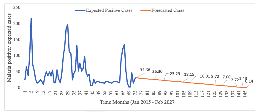
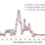
In the context of malaria transmission in Masvingo district, the parameter values chosen are shown in Table 4[22], and the following initial conditions were selected: and the best model fit, determined by the square of the Pearson’s product moment correlation coefficient ( passing through the data provided is shown in Figure 2. RDNS- positive cases (infected) refers to the individuals who tested malaria positive and notified according to the Rapid Disease Notification System (RDNS). Expected malaria cases were obtained after applying the model to the existing disease data (cases), to see how best it fits the data. The 2-period moving average was obtained by finding the average of two consecutive values which seeks to smooth-out month-to-month fluctuations.
The trend in the incidence of malaria over time is shown. Although there is a general decline in the number of malaria cases, the transmission dynamics is highly fluctuating (Figure 2).